Fixing disabled wireless on Lenovo Z360 running Ubuntu 10.10

Ok, this post isn't about chemistry at all. However, I'm going to defend it under the category of free software. Here is a short introduction to my problem. I have a Lenovo Z360 laptop running Ubuntu 10.10. It came with some Windows distribution (are they even called distributions? I haven't had a windows computer since 2004) which I never used. <sarcasm> Thanks to Lenovo, the laptop was set up with some proprietary driver software for my wireless network interface card (NIC). </sarcasm>

After installing Ubuntu 10.10 (AKA the perfect 10) everything was working fine ... until I one day pressed the "turn off wireless" buttons (Fn+F5) to save a tiny amount of battery power. This apparently bypasses the hardware "disable wireless switch" and switches off wireless via some built-in firmware. And since I wasn't using the proprietary drivers in Windows, there was no way to switch wireless back on. 

The tedious solution to my problem was to replace the solid-state drive I had put in myself for the original drive, and boot up in windows, switch on wireless using the proprietary driver software. 

Long story short, I have up until this day always been carrying the original harddive and a small screwdriver with me, in case I should accidentally turn off wifi, so I could perform the wireless-enabling surgical procedure.

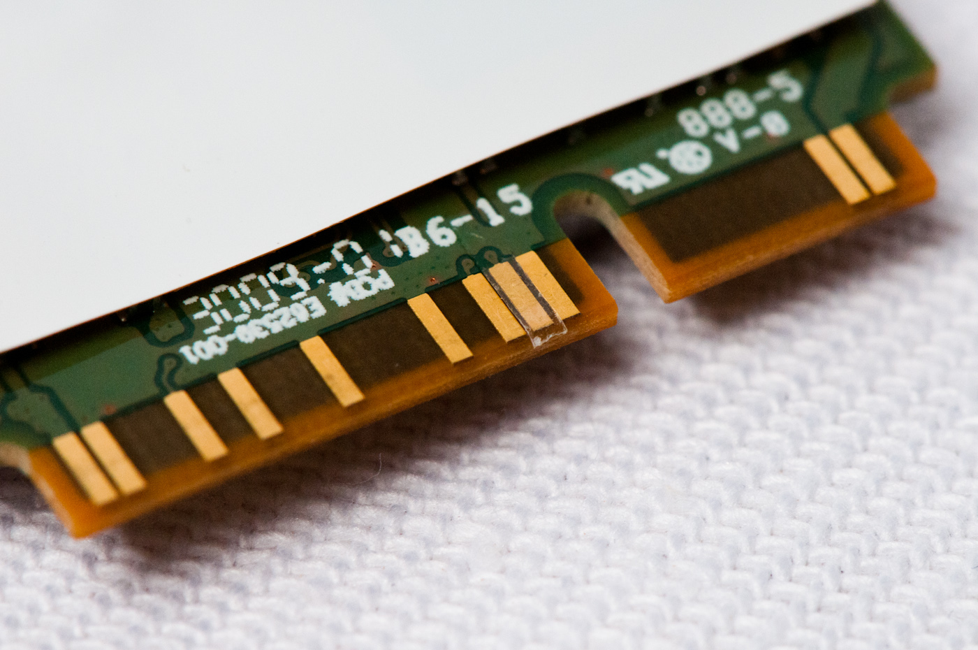
However, today I stubled up a more permanent solution. I turns out, that the signal to turn off the wireless NIC is transmitted via pin #20. So to avoid ever turning off wireless you just have to tape over that particular pin - see the picture below. After five minutes of fiddling with tape, tweezers and scissors I managed cut a piece of tape small enough and put it precisely over the pin. 

And lo and behold - it's now impossible to disable the wireless NIC via switches or accidental key-presses!

Thanks to the guys over at anandtech.com for pointing this out! And thanks to Lenovo for this post possible by making hardware that just works out-of-the-box-until-it-doesn't-and-there's-no-way-to-switch-it-back-on-besides-software-only-written-for-one-particular-operating-system.

Code snippets on blogs

I had a brief discussion with Casper Steinmann about how to present code snippets in blog-posts. We both agreed that nice formatting is really important. We also agreed that our previous attempts to do so were (and still are) crummy.

One of the (easy) ways to set up nice formatting can be found over at CraftyFella:

http://www.craftyfella.com/2010/01/syntax-highlighting-with-blogger-engine.html

Just put some stuff in your blogger template and all you have to do is wrap your code examples in HTML <pre>  tags. "Pre tags" denote a pre-defined format, and are often used to wrap around code examples, with the color coding pertaining to that particular code-language and an equispaced font, which makes it possible to use indentations properly.

Most popular programming languages are supported in this method. C, C++ C#, python, and probably many others. Hoever, no support for FORTRAN - quantum chemists beware. If you know of a user-friendly syntax highlighter that does FORTRAN, do leave a comment! Everybody loves FORTRAN.

Here is a simple example of how a dumb python script looks after using CraftyFella's guide to set things up:

#!/usr/bin/python

def print_string(string):
    print string

hello_world = "Hello world, look at my fancy code formatting!"

for i in range(10):
    print_string(hello_world)

... and a little bit of C++:

//! Return size of collection
//! \return size of collection
unsigned int size() const {
     return data_vector.size();
}

Molecular dynamics and supercomputing, past and present

What is the most powerful single computer you can get today, measured in sheer numbers of double precision floating point operations per second (flops)? Possibly, the answer is a rack server (such as the HP half-width 4U in the picture below) with no less than eight(!) Nvidia Tesla M2090 cards installed. Each card offers a theoretical max of 665 Gflops of double precision computing power -- a total of 5.3 Tflops (not counting any CPUs). Now, go to the Top500 and find the list from 10 years ago ... November 2001. Just one of these servers would bring you a safe 3rd place on the list - very impressive for just ONE single machine.

Foto

One might argue, that a 4U rack unit is not a very practical computer - so what's the max you can cram into a a standard sized ATX chassis these days? Well, take four of these GPUs (and a good power supply), and you're up to about 2.7 Tflops, theoretical peak. 10 years ago that would bring well into top10 world wide with a box that you could put under your desk!

The Japanese "K Computer" is currently the fastest cluster out there and recently broke the 10 Pflops barrier (10¹⁶ flops)! Now, he question is, when can I expect to have that kind of performance in a desktop PC, and how about my huge ms protein molecular dynamics simulation?

Speculating on the future is difficult, so I'm just going to "re-blog" this review paper I stumbled upon by Michele Vendruscolo and Christopher M. Dobson, "Protein Dynamics: Moore’s Law in Molecular Biology", Current Biology, 21, R68-R70 (2011), which speculates on the future of MD simulations. According to the authors, MD computing power sees exponential growth, so hopefully, I can one day have a 10 Pflops (I'm willing to settle for less) box under my desk. Here are some of the bold predictions from the paper:

• In 2010 we saw the first nanosecond scale MD simulation of the Ribosome

• In 2030 we'll be moving up to millisecond  scale MD simulation of the Ribosome
• in 2050 we'll be doing all-atom dynamics of entire bacteria on a nanosecond scale.

I can't wait to get older and see an all-atom bacteria simulation!

Compiling DALTON2011 with 64-bit integers, OpenMPI and MKL

I was asked if I could do a blog post about how to compile DALTON2011 in parallel with 64-bit integers. This is not entirely trivial, unless you know what's going on. One of the key ingredients is an MPI that supports 64-bit integers, which OpenMPI does not do out of the box. I found 64-bit integers required to complete all test cases succesfully. This tutorial will assume that you have a working set of Intel compilers.

1) Get the OpenMPI 1.4.3, which is the latest stable version to support 64-bit integers:

wget http://www.open-mpi.org/software/ompi/v1.4/downloads/openmpi-1.4.3.tar.bz2

tar xjf openmpi-1.4.3.tar.bz2

cd openmpi-1.4.3/

2) Now you're ready to compile OpenMPI. I keep my compiled programs in ~/programs/ -- you can use whatever directory you want, so change the prefix to wherever you want it. If you have root access /opt/ would be a great place to put OpenMPI. First, export the CXX, CC, FC and F77 environment variables to specify that you want to use the dedicated Intel compilers. Then run the configure script with the -i8 flag, specifying support for 64-bit integers:

export CC=icc; export CXX=icpc; export FC=ifort; export F77=ifort

FFLAGS=-i8 FCFLAGS=-i8 ./configure --prefix=/home/andersx/programs/openmpi-1.4.3/

make

make install

(both configure and make can take quite a while)

3) Now, you need to export the following variables:

export PATH=/home/andersx/programs/openmpi-1.4.3/bin:$PATH

export LD_LIBRARY_PATH=/home/andersx/programs/openmpi-1.4.3/lib:$LD_LIBRARY_PATH

You can also add these lines to you ~/.bashrc file, but I wouldn't recommend this, since you might want another version of OpenMPI for another program, so it's better to only export the variables you need, when you actually need them.

Check that your compiled OpenMPI is working by typing:

which mpirun

This should return something like (in the folder you specified in the --prefix in step 2):

/home/andersx/programs/openmpi-1.4.3/bin/mpirun

Further more, check that your OpenMPI picked up the -i8 flag properly (the compiler flag that tells to compile for 64-bit integers):

ompi_info -a | grep 'Fort integer size'

This must return size 8:

         Fort integer size: 8

If not, you did something wrong, and the following steps will not work!

4) Go to http://dirac.chem.sdu.dk/daltonprogram.org/www/download.html and download the latest version. Untar it, and head into the DALTON2011 folder:

tar xjf Dalton2011_release_v0.tbz

cd Dalton2011_release/DALTON/

Start the configure script and answer the following questions with:

This appears to be a -linux architecture. Is this correct? [Y/n] y

Do you want 64-bit integers? [y/N] y

Do you want to install the program in a parallel MPI version? [Y/n] y

Compiler /home/andersx/programs/openmpi-1.4.3/bin/mpif90 found, use this compiler? [Y/n] y

(This must be found in the folder where you just compiled and installed OpenMPI in steps 1-3)

Compiler /home/andersx/programs/openmpi-1.4.3/bin/mpicc found, use this compiler? [Y/n] y

(This must be found in the folder where you just compiled and installed OpenMPI in steps 1-3)

Do you want to replace this with your own directory search list? [y/N] n

(Just install whatever BLAS/LAPACK the script finds .. we're going to use MKL, but we need to specify that manually later on, overriding what the script finds here)

The remaining questions you can answer however you want to.

5) Now we need to find out, where MKL is placed on you system. This may vary from version to version of the Intel Compiler suite. First write:

env | grep MKL

This returns something like:

MKLROOT=/opt/intel/composerxe-2011.0.084/mkl

If it doesn't, you haven't got the Intel Compilers (and MKL) properly installed. Now head into this directory and locate libmkl_intel_ilp64.a:

cd $MKLROOT

locate libmkl_intel_ilp64.a

This returns something like:

/opt/intel/composerxe-2011.0.084/mkl/lib/intel64/libmkl_intel_ilp64.a

The above directory we will call MKL_LIB_DIR:

export MKL_LIB_DIR=/opt/intel/composerxe-2011.0.084/mkl/lib/intel64

Last thing in this step is to edit the Makefile.config and put the information we now have into it. Open Makefile.config with your favourite editor and replace the line that starts with "LIBS = " with:

LIBS = -L/usr/lib -lmkl_lapack95_ilp64 -Wl,--start-group $(MKL_LIB_DIR)/libmkl_intel_ilp64.a $(MKL_LIB_DIR)/libmkl_sequential.a $(MKL_LIB_DIR)/libmkl_core.a -Wl,--end-group -lpthread

(the above is all in one line)

This will link to the correct MKL library, which supports 64-bit integers (also why they're called ilp64) and made for the Intel compilers. Now it's a good time to make sure that you still have the environment variables from step 3) exported. So now we're ready to actually compile DALTON2011:

make

(now it's time to get a coffee, and do something else for a long while ... Also compiling DALTON2011 does not seem to work in parallel so no -j8 flags here!)

6) Compiling ends without errors and the following line:

mv ./dalton_mpi.x /home/andersx/zips/Dalton2011_release/bin/dalton_mpi.x

To test your compilation head into the test/ folder and start testing the parallel (these only take a minute or so .. the full test suite takes much longer).

cd test/

./TEST parallel

Hopefully this returns:

#####################################################################
                              Summary
#####################################################################

ALL TESTS ENDED PROPERLY!

date and time         : Sat Oct 29 10:54:20 CEST 2011

If not, something is wrong. :) Now proceed to the full test suite. I use nohup and just check the output in nohup.out.

nohup ./TEST all &

less nohup.out

Hopefully nohup.out end with (after an hour or so):

All tests completed successfully
Perl-style tests computed successfully

Perl-style tests finished!

#####################################################################
                              Summary
#####################################################################

ALL TESTS ENDED PROPERLY!

date and time         : Sat Oct  29 13:02:34 CEST 2011

This means DALTON2011 works!

You can also head over to the DIRAC10 wiki pages, which is very much like compiling DALTON: http://wiki.chem.vu.nl/dirac/index.php/Installation_guide

For support go to: http://dirac.chem.sdu.dk/daltonprogram.org/www/docs.html

I did this on a Intel Core i5-760 with Ubuntu 10.04.3 Server and Intel Compilers version 12.0.0 20101006. The entire test suite took twice as long compiling with GNU compilers, so I recommend staying away from these for a "production" version. Further more MKL is one of the fastest and most stable BLAS and LAPACK libraries there is and it comes precompiled for 64-bit integers with the Intel Compilers, so do use MKL and save yourself a headache! Also GNU compilers >4.4 have compiler issues from what I've heard.

Fast Lennard-Jones and electrostatics on a CPU

I recently got interested in programming molecular mechanics force fields on CPUs and GPUs. One of the hurdles you have to get through, is the non bonded interactions, which you have to iterate over all pairs of atoms. It thus scales as N^2 with the number of atoms, whereas the bonded terms scale only linearly. A good example is the OPLS force field (read more on Wikipedia). Here the non-bonded interactions are given by a Lennard-Jones potential term an an electrostatic term:

For more information about molecular modeling and force fields, I can  recommend reading the Molecular Modeling Basics book, which has excellent pages on the subject. You can also just ask in the comment sections, if you have anything. Finally, the code can be found for download at the bottom of this post.

Now let's get started! I've put the coordinates of all atoms in the double coordinates[] 2D array. In the example I'm using the coordinates of the protein structure of Cutinase 1CEX, which has 2867 atoms. I used pdb2pqr for protonation. I'm going to assume (for simplicity), that all interactions use the same parameters. The naive way to implement the non-bonded OPLS interaction could be (in C/C++):

// Lennard-Jones parameters
double A = 10.0;
double C = 10.0;
// Electrostatic parameter
double E = -10.0;

double non_bonded_interaction(const double a[3], const double b[3]) {

     // Fastest way of getting distance
     double distance = sqrt((a[0] - b[0]) * (a[0] - b[0])
                          + (a[1] - b[1]) * (a[1] - b[1])
                          + (a[2] - b[2]) * (a[2] - b[2]));

     return A*pow(distance, -12.0) 
          + C*pow(distance, -6.0)
          + E/distance;
}

int main() {

     // Set energy to 0
     double energy = 0.0;
     // Loop over all atoms
     for (unsigned int i = 0; i < n_atoms; i++) {

          // Only up to i-1, to avoid double counting 
          // interactions, and self-interactions
          for (unsigned int j = 0; j < i; j++) {

               energy += non_bonded_interaction(coordinates[i],
                                                coordinates[j]);

          }
     }
     std::cout << "E = " << energy << std::endl

     return 0;
 }

Timing this gives 0.0300 µs per iteration with the Intel icpc compiler, and 0.189 µs with the g++ compiler, both with -O3 optimization. 

As I will demonstrate, this is because pow() is horribly implemented in g++. Lets further optimize the non_bonded_interaction() function:

double non_bonded_interaction(const double a[3], const double b[3]) {

     double distance = sqrt((a[0] - b[0]) * (a[0] - b[0])
                          + (a[1] - b[1]) * (a[1] - b[1])
                          + (a[2] - b[2]) * (a[2] - b[2]));

     double distance6 = distance * distance * distance
                      * distance * distance * distance;
     double distance12 = distance6 * distance6;

     return A/distance12 + C/distance6 + E/distance;
}

Now we get: 0.0295 µs with icpc and 0.0313 µs with g++. Clearly pow() shouldn't be used with GNU compilers!

Next on our list of optimizations is getting rid of divisions. Divisions are performed iteratively by the CPU, while multiplications are done bit-parallel by specialized circuits hard-coded into the CPU silicon. We have three divisions, but we can write everything in terms of only one, using reciprocal distances:

double non_bonded_interaction(const double a[3], const double b[3]) {

     double distance = sqrt((a[0] - b[0]) * (a[0] - b[0])
                          + (a[1] - b[1]) * (a[1] - b[1])
                          + (a[2] - b[2]) * (a[2] - b[2]));

     double inv_distance = 1.0/distance;
     double inv_distance6 = inv_distance * inv_distance
                          * inv_distance * inv_distance
                          * inv_distance * inv_distance;
     double inv_distance12 = inv_distance6 * inv_distance6;

     return A * inv_distance12 
          + C * inv_distance6 
          + E * inv_distance;
}

This gives us 0.0173 µs with icpc and 0.0189 µs with g++. Still ... there is one division left and also a square-root which is problematic. These are what takes up by far the most time in the calculation. But there is a hacky trick we can use. I'm going to show you how to use an approach by Newton to estimate inverse square roots .. take a look at this Wikipedia page for more info. The method became famous after it was found in the Quake III open source engine. Here it is in double type, so slightly different than the float type example on wikipedia. I'm using two final iterations to achieve sufficient accuracy.

inline double fast_inv_sqrt(double number) {

        long long i;
        double x2, y;
        const double threehalfs = 1.5;
        x2 = number * 0.5;
        y  = number;
        i  = * ( long long * ) &y;
        i  = 0x5fe6ec85e7de30da - ( i >> 1 );
        y  = * ( double * ) &i;
        y  = y * ( threehalfs - ( x2 * y * y ) );
        y  = y * ( threehalfs - ( x2 * y * y ) );
        return y;
}

Using this, we can avoid ever dividing and taking square roots, and reduce our code to:

double non_bonded_interaction(const double a[3], const double b[3]) {
     double dx = (a[0] - b[0]);
     double dy = (a[1] - b[1]);
     double dz = (a[2] - b[2]);
     double distance_sqr = dx*dx + dy*dy + dz*dz;

     double inv_distance   = fast_inv_sqrt(distance_sqr);
     double inv2_distance  = inv_distance * inv_distance;
     double inv6_distance  = inv2_distance * inv2_distance
                           * inv2_distance;
     double inv12_distance = inv6_distance * inv6_distance; 
     return A * inv_distance12 
          + C * inv_distance6 
          + E * inv_distance;


}

Now, timings are down to 0.0118 µs for icpc and 0.0155 µs for g++ per iteration. It's hard to optimize the code further from here, using code that isn't very hacky, but we still got a x2.5 times speed-up with the Intel compiler and x12.2! times speed-up with the GNU C++ compiler. Still, we can always try and parallelize the code using OpenMP. This is the easiest way to parallelize code there ever was. We only need to add ONE compiler flag, which tells it to parallelize the next loop. Take a look:

// Loop over all atoms
     for (unsigned int i = 0; i < n_atoms; i++) {

// Tell compiler, to run next in loop in parallel
#pragma omp parallel for reduction(+:energy)

          //Only up to i-1, to avoid double counting interactions, and self-interactions
          for (unsigned int j = 0; j < i; j++) {

               energy += non_bonded_interaction(coordinates[i], coordinates[j]);

          }
     }

To compile we also must remember to link to OpenMP:

icpc -O3 cpuff.cpp -o cpuff -openmp (for Intel)
g++ -O3 cpuff.cpp -o cpuff -fopenmp (for GNU)

On four cores instead of one, this gives us: 0.0042 µs for icpc and 0.0042 for g++ as well. That's a x2.8 and x3.6 speed up for Intel and GNU, respectively! Not too shabby, by no means! Compared to the unparallelized code, this is a x7.1 speed-up for Intel and a whooping x45.0 speed-up for the initial lazy GNU compiled code.

I hope this post will inspire you to play around with these easy-to-do optimizations yourself. You can download code examples here:

cpuff.cpp (the implementation)

coordinates.h (the protein coordinates. I put this in a 2D array to avoid writing a parser)

DISCLAIMER: The above was carried out on an Intel Core i5-760 running 64-bit Ubuntu Server 10.04.3, icpc (ICC) 12.0.0 20101006 and g++ (Ubuntu 4.4.3-4ubuntu5) 4.4.3. Timings are averages over 10 consecutive runs. I compiled everything with -O3 optimization.

C++ timing with millisecond accuracy

How do you know if you have efficiently implemented a routine. A simple routine from Boost can tell you. More specifically the boost::timer function.
Boost is a set of free software libraries that extend the functionality of C++, in the Wikipedia discription. There are tons of very useful features you'd expect to be native to an advanced programming language as C++ but are not.

How to get boost? Usually on Linux you can just say something like apt-get install libboost or yum install libboost. Let me know if you want a tutorial to compile or install boost. The examples below compile with both Intel and Gnu C++ compilers and even Nvidia compilers (I tried NVCC 4.0).

Here is a code example of how to time a routine with boost:

#include <boost/timer.hpp>      // For boost::timer class
#include <iostream>             // For printing


// Some constants
unsigned int x = 20000;
bool flag = true;
unsigned int k = 0;

int main() {
        // Start boost timer.
        boost::timer t;

        // Do a double loop that takes some time.
        for (unsigned int i = 0; i < x; i++) {
                for (unsigned int j = 0; j < x; j++) {
                        k = i + j;
                        if (k % 2 == 0) {
                                flag = false;
                        } else {
                                flag = true;
                        }
                }
        }

        // Store elapsed time from boost
        double elapsed = t.elapsed();

        // Print elapsed time from the t object.
        std::cout << "boost/timer says:" << std::endl;
        std::cout << "Total time    = " << elapsed 
                << " seconds" << std::endl;
        std::cout << "Avg time/iter = " << elapsed / (x * x) 
                << " seconds" << std::endl;

        return 0;
}

I get the following output on my Core i5-760 box and the icpc compiler:

boost/timer says:
Total time    = 0.35 seconds
Avg time/iter = 8.75e-10 seconds


You can use t.reset() if you want to reset the timer in your program.


If you want higher accuraccy, you can use the gettimeofday() function from sys/time.h. This example does not require boost either, but the code is way uglier. This is done very much like in the above code:

#include <sys/time.h>           // For gettimeofday()
#include <iostream>             // For printing


// Some constants
unsigned int x = 20000;
bool flag = true;
unsigned int k = 0;

int main() {

        // Create objects for gettimeofday() timing
        struct timeval start_time;
        struct timeval end_time;

        // Get the time of day -- NULL means we don't care about
        // time zones. Store in start_time.
        gettimeofday(&start_time, NULL);


        // Do a double loop that takes some time.
        for (unsigned int i = 0; i < x; i++) {
                for (unsigned int j = 0; j < x; j++) {
                        k = i + j;
                        if (k % 2 == 0) {
                                flag = false;
                        } else {
                                flag = true;
                        }
                }
        }

        //Store time of day in end time
        gettimeofday(&end_time, NULL);

        // Calculate the elapsed time with micro second accuracy from gettime of day
        double start = start_time.tv_sec*1000000 + (start_time.tv_usec);
        double end   = end_time.tv_sec*1000000 + (end_time.tv_usec);
        elapsed     = end - start;

        // Print elapsed time from gettimeofday().
        std::cout << "gettimeofday says:" << std::endl;
        std::cout << "Total time    = " << elapsed 

                << " microseconds" << std::endl;
        std::cout << "Avg time/iter = " << elapsed / (x * x) 

                << " microseconds" << std::endl;

        return 0;
}

This gives me the following output:

gettimeofday says:
Total time    = 366208 microseconds
Avg time/iter = 0.00091552 microseconds

Happy coding! Let me know if you have questions or comments.

HOWTO: Mixed basis In Gaussian

One of the many tricks in speeding up quantum chemistry calculations is the use of locally dense basis sets. Maybe it is only necessary to have diffuse functions on certain atoms or you may only need to calculate parts of a system with a high accuracy.

Use of locally dense basis sets is completely legal within the basis set approximation. Just remember, that things like Mulliken charges will often be off, if some atoms have significantly more basis functions than other.

In this example an example, I show how to do a geometry optimization a of methylamine at the Hartree-Fock level of theory with a 6-31G basis set on carbon and nitrogen and a 3-21G basis set on hydrogen atoms. Note that the basis set is specified as "gen". This option tells Gaussian to use the basis set specified at the bottom. A the bottom there is a number for each atom (followed by a 0 for reasons unknown to the author), and the name of the basis set below. Data for each atom is terminated by a line containing four asterisks.

Remember to separate "groups" of data with exactly one blank line and the file must be terminated with exactly two blank lines.

--------------------------Start of file--------------------------

# opt hf/gen geom=connectivity

Title Card Required

0 1

 C                 -7.52265887    1.01208458    0.00000000

 H                 -7.16600444    0.00327457    0.00000000

 H                 -7.16598603    1.51648277   -0.87365150

 H                 -8.59265887    1.01209776    0.00000000

 N                 -7.03265039    1.70504284    1.20025020

 H                 -6.03265041    1.70487221    1.20034129

 H                 -7.36582334    2.64790856    1.20015900

 1 2 1.0 3 1.0 4 1.0 5 1.0

 2

 3

 4

 5 6 1.0 7 1.0

 6

 7

1 0

6-31G

****

2 0

3-21G

****

3 0

3-21G

****

4 0

3-21G

****

5 0

6-31G

****

6 0

3-21G

****

7 0

3-21G

****

--------------------------End of file--------------------------