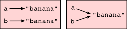
I can never correctly remember when things are passed as references or copied as local variables inside functions.
Take these two, innocuously looking functions. Because both do the same thing (namely set the contents of a vector, P, to [1, 1]) I call them 1 and a, respectively, since one is not better than the other.
def implementation_1(P):
P = [1, 1]
def implementation_a(P):
P[0] = 1 P[1] = 1
What you would expect is one of the following two options
Both functions change P to [1, 1] (permanently).
Both functions take a local copy of P and change it to [1, 1], and after the function returns, the local [1, 1] array is forgotten.
A simple test is to do this:
P = [0, 0] print P
implementation_1(P) print P
implementation_a(P) print P
which prints:
[0, 0] [0, 0] [1, 1]
So clearly implementation_a() is different from implementation_1(), although they seemingly do the same.
This is taken from a lecture I gave during the Molecular Statistics course at University of Copenhagen, which I co-teach with +Jan Jensen and +Jimmy Kromann. The students have to program different types of molecular simulations and are not expected to have any programming experience before the course.
Random walk Monte Carlo seems a bit silly at first glance, since a simulation does not really contain a lot of information. As the name implies, the motion of the particle is completely random, much like Brownian motion of a particle suspended in a fluid. The behavior of a particle in a random walk simulation is very much like the movement of the average particle in a fluid, which randomly and constantly bounces into other particles, every time from a random direction.
A collection on particles will then have average properties much like a liquid or (as we have looked a lot at in the course) the Lennar-Jones fluid. Do note, that there are no interactions between any particles.
A simple one-particle random walk Monte Carlo simulation is shown here.
The equations of motion are shown here:
$$x(t + dt) = x(t) \pm \mathrm{random.random()} \cdot \mathrm{d}l $$
$$y(t + dt) = y(t) \pm \mathrm{random.random()} \cdot \mathrm{d}l $$
where random.random() is the Python default random number generator and $\mathrm{d}l$ is a scaling factor that determines the average step-length. The fact that the equation does not include any interaction terms makes it computationally cheap to simulate a lot of particles.
In the last Molecular Statistics class we used random walk Monte Carlo to obtain the diffusion coefficient via Fick's second law, here in one dimension:
$$\frac{\partial \phi}{\partial t} = D\ \frac{\partial^2 \phi}{\partial x^2}$$
The solution of Fick's second law is a Gaussian function
$$\phi (x, t) = \frac{1}{\sqrt{2\ \pi\ \sigma^2}} \exp \left( - \frac{x^2}{2 \sigma^2}\right)$$
with $\sigma = \sqrt{2\ D\ t}$. So if we can calculate $\sigma$ from the distribution of particles, we can immediately get the diffusion coefficient.
The simple approach is to start a random walk simulation with many particles and then fit the distribution of particles to a Gaussian.
We used this extremely simple Python/Numpy program to simulate random walk and calculate $D$:
X = numpy.zeros(n_particles)
for i in range(n_steps):
X += numpy.random.uniform(-dl, dl, n_particles)
sigma = X.std()
print "D =", sigma**2 / ( 2 * i)
The simulation looks like this in 2D (with 400 particles):
As you can see, the particles collectively look like they are diffusing through a medium. The diffusion constant is the derived (here only in the $X$-direction by fitting the distribution to a Gaussian function (which was simpy done via Numpy's .std() function). The time evolution of the distribution of particles (blue histogram) and the Gaussian fit (red curve) looks like this:
The time evolution of $D$ should converge pretty quickly. You can see $D$ for a simulation with 10,000 particles below. It took a matter of seconds on Jimmy's old laptop to run this. Imagine doing an long enough MD with 10,000 particles on your laptop!
This is a concept that has annoyed many a newcomer to Python - including the author of this post. I will be talking briefly about this concept in my lecture next Thursday, and the excellent TA, +Jimmy Charnley Kromann, pointed me to an example he saw on pythontutor. The Visualize tool on pythontutor is a very explicit way to illustrate what happens under the hood of python: http://www.pythontutor.com/visualize.html
If you want to avoid pointer aliasing, you usually want to do one of these three things in order to copy a to b:
1) b = a[:]
This takes a shallow copy. Personally, I don't like this option, because the slicing notation is not clear to everyone. But it is definitely the shorter notation. This will fail if you want to copy a list of lists. Being a shallow copy, it does not copy lists of lists. It will merely copy the list of pointers to other "sub"-lists.
2) import copy b = copy.copy(a)
This takes a shallow copy. It is more clear from the code what this does, so this is usually my preferred approach. Still a shallow copy, however.
3) import copy b = copy.deepcopy(a)
This is the fail-safe method and takes a copy of everything, so use this if you're in doubt. Works pretty much in every case. The down side is that it's usually slower to copy everything with deepcopy.
I've started using Numba to speed up MD simulations for our course in Molecular Statistics, which I teach together with +Jan Jensen and +Jimmy Charnley Kromann.
One exercise is using the Velo-Verlet algorithm to simulate a Lennard-Jones gas/liquid with periodic boundary conditions. Since we do everything in Python in this course, running the actual simulation is quite slow. What we do is we supply the students with a compiled FORTRAN module, compiled with F2PY which they can use when they've written their own Lennard-Jones gradient code.
The FORmula TRANslator module is extremely fast, compared to Python code. I rewrote the code from last year's course to a function I could use with Numba and compare directly to the F2PY module
For 100 particles:
Numba: 0.146 ms/iteration (466x speed up)
F2PY: 0.236 ms/iteration (289x speed up)
Python: 68.06 ms/iteration
Now, I'm pretty sure a pure FORTRAN implementation would be faster than the F2PY, but I am very impressed with the Numba, since it's standard Python code and MUCH more simple to read than FORTRAN -- in theory all you have to do is write @autojit before a function definition. This is of course in theory ... I didn't do anything to improve on the readability of the Lennard-Jones code here. Before I posted, I had actually inserted a comment saying """This code block is unreadable""".
Now, there were a few issues I discovered:
1) @autojit vs. @jit(argtypes=[double[:,:], double[:]])
Since Numba has to decide what arguments a function takes before it's being compiled, it needs to know what possible type of arguments the function takes. If you're lucky, Numba decides on the right type and you can get away with @autojit, but sometimes autojitting makes the code SLOWER than standard, interpreted Python. In one case I got a factor of 10x slower with autojit, but explicitly stating the function argument types with @jit(argtypes = .... ) I got a speed up of 20x on the same code compared to interpreted Python.
2) Returning tuples in compiled code block
Numba does not allow a tuple to be returned inside a compiled code block. So don't do this.
3) Use Numpy properly
Numba is NumPy aware, so code ran faster when numbers were stored in numpy.array types rather than just regular Python lists.
At first I was numpy.round() to round to nearest integer in the periodic boundary condition code. Switching three numpy.round() calls to numpy.rint() gave a speed up of around 100x on the code execution.
Use U[i, j] instead of U[i][j] on NumPy arrays. Not much of a difference in the vanilla Python code, but MASSIVE speed gains in compiled code.
I am currently teaching the Molecular Statistics course together with +Jimmy Charnley Kromann and +Jan Jensen at the University of Copenhagen. My part of the course is teaching the students how to program simple molecular simulation algorithms in Python. +Jan Jensen does the theoretical lectures, and I give lectures in basic Python programming and how to implement the equations from Jan.
One of the challenges we faced before the start of the course was to just get Python, Numpy and Matplotlib up and running on every single student's laptop. Since the students run everything from Windows XP, 7 and 8 to Linux and Mac, this can pose quite a challenge for the students, some of which have barely ever even installed a program before.
This year, we opted to create a VirtualBox with Ubuntu on it, and make sure everything the need throughout the course was pre-installed. The students could then simply download the VirtualBox program and install our VirtualBox image.
+Jimmy Charnley Kromann made this excellent video of how to get the VirtualBox going before the first class:
My biggest fear was that the students would be frightened and confused by their first meeting with a non-Microsoft system. But that (fortunately!) didn't turn out to be an issue at all.
These are my observation from the first lecture and first exercises class:
To my surprise all of the students had managed to bring their laptop with a working VirtualBox to the first class. ALL students! I was pretty thrilled since that meant they all could follow my programming from the projector on their own laptop, which is what I want them to do during my lectures.
What was going on on the projector was the same as on their laptop during the lecture, which I think help lessen the confusion.
We didn't have to do ANY tech support during the interactive lectures or the following exercises class to get Python working. Only hitch was two students who wanted American keyboard layout (our Box came with a Danish keyboard layout by default). This was quickly (though some might say awkwardly) solved by "setxkbmap us" in the terminal.
Some of the groups of students wanted an extra module to make a video of the things they had plotted in Matplotlib. +Jimmy Charnley Kromann then posted simple instructions and the relevant "sudo apt-get install" command on the course website -- so that went relatively easy as well.
Things which didn't work very well were the shared clipboard
and drag-and-drop of files between the host OS and the VirtualBox. That
only worked on 50% of the student's laptops. Must be a bug in VirtualBox
somewhere.
I only overheard the sentence "Grrr, I hate linux!" once.
I'm teaching a course in molecular simulations this year in which the students have to program simulations of various simple systems. We're trying to keep things as simple as possible and everything is done in Python.
The task of the second week of the course is to program a simple simulation of a 2D Lennard-Jones gas. The computationally intensive step in this exercise is calculating the energy and gradient. In the past we've (and by we, I mean +Casper Steinmann) written a FORTRAN module and used F2PY to exploit the awesomeness of the good old FORmula TRANslator and have the students link their Python scripts with a precompiled .so module for this to run at an acceptable speed
This solution is of course completely fine, but not very general. I've been looking into Cython, pypy and various other methods to speed things up a bit. But they all seemed quite elaborate an unPythonic, and you might as well do the whole thing in C then.
Yesterday Numba was brought to my attention on this blog. In short, Numba is a way to compile (at execution time) Python functions into C which normally makes your program run substantially faster. The blog has a very nice example where the code gets a 1000x speedup just by adding one function decorator. And the syntax couldn't be simpler.
Let's try Numba on our Lennard-Jones program. Here is the naive function they have to implement:
The code is then executed via Python as one would normally execute Python code, specifying in the script that the calc_energy_and_gradient() function is to be compiled via Numba. This can be done simply by writing the the @autojit decorator before the function definition.
You can also specify exactly which type of input the just-in-time compilation takes takes (an example is commented out). This makes the compilation of the function be type specific, but a bit faster. Make sure to import numba and the specific type of argument (here the arguments are of the type double) and the relevant decorators (jit or autojit).
Conclusion: 10000 gradient and energy evaluations take 16 seconds with the standard Python implementation. 2 seconds with @autojit and 1.5 seconds with the explicit @jit. Not too bad for something that doesn't take ANY code changes.
I am looking at the conversion of chorismate to prephenate in Chorismate Mutase, to benchmark a hacky EFMO-RHF:MP2 method we've implemented in our group. Casper Steinmann did an adiabatic mapping of the reaction path, and we though it'd be cool to do coupled cluster single point energies on snapshots from the reaction path and some something ONIOM style.
Figure 1: Snapshot 1 from the reaction path; chorismate to prephanate
Anyways, the reaction complex contains 118 electrons, so we fired up MOLPRO2012 and started looking at the DF-LCCSD(T0)-F12a method. A name you should probably memorize from now on.
The single point energy evaluation took 3:43 hours with the VDZ-F12 basis set! Mind you, this was on only a single CPU core with 4 GB 16GB of RAM allocated, so no supercomputers were involved.
First I though the calculation had crashed because it didn't show up in the queue. My first attempt with the 3-21G basis set didn't converge because I failed to set the charge to -2, but this time around Molpro actually gave me an energy!
Next problem on my list is to calculate the good old MP2/cc-pVTZ energy I need to subtract in order to get my ONIOM results. Those are going to take about 5-10 hours on 8 cores.
This is what the input file looked like for anyone interested
memory,2000,M geomtyp=xyz geometry 24 NS= 27 NA= 105 NF= 9 EFMO2-RHF:MP2 (this line is just a title btw) C 42.243912717439 56.985332654358 33.508219032291 O 44.083656765173 58.469818126062 33.547456767374 C 42.170657938422 56.969234127412 32.053802633762 O 43.705108088223 57.205919113255 35.368497584787 C 41.129420410826 56.416380137206 31.405612518418 O 36.855437867615 57.552564896356 32.240095659821 C 40.011578869479 55.731334232825 32.133332774369 O 37.952282803211 59.164070642440 31.158486994867 C 39.926225853593 56.110094283828 33.626395940165 O 40.227454849874 54.351343596304 31.951217705746 C 41.196604656028 56.578036178752 34.246569733982 O 38.910804760126 57.082428023235 33.866893577924 C 38.968148927395 58.213925767965 33.092045796028 C 39.831866096203 59.221137407117 33.269727518172 C 43.428858040104 57.602185825538 34.190487998445 C 37.845543926101 58.319486314173 32.113613710711 H 39.478451838017 53.847769952241 32.300919500400 H 39.060609728200 56.030078213449 31.676260590468 H 39.584331039092 55.233181854460 34.161137739114 H 41.108061134298 56.387696261961 30.326013340305 H 42.988978401897 57.425894863516 31.511012407792 H 41.233442365036 56.630502649395 35.323808064193 H 40.574407364526 59.218144574703 34.050005215454 H 39.764972282572 60.084246967681 32.627123054496 end
Thomas B. Adler, Hans-Joachim Werner (2011) "An explicitly correlated local coupled cluster method for calculations of large molecules close to the basis set limit" J. Chem. Phys. 135, 144117; http://dx.doi.org/10.1063/1.3647565